Pareto efficiency
Pareto efficiency, or Pareto optimality, is a concept in economics with applications in engineering and social sciences. The term is named after Vilfredo Pareto, an Italian economist who used the concept in his studies of economic efficiency and income distribution.
Given an initial allocation of goods among a set of individuals, a change to a different allocation that makes at least one individual better off without making any other individual worse off is called a Pareto improvement. An allocation is defined as "Pareto efficient" or "Pareto optimal" when no further Pareto improvements can be made.
Pareto efficiency is a minimal notion of efficiency and does not necessarily result in a socially desirable distribution of resources: it makes no statement about equality, or the overall well-being of a society.[1][2]
Contents |
Pareto efficiency in short
An economic system that is not Pareto efficient implies that a certain change in allocation of goods (for example) may result in some individuals being made "better off" with no individual being made worse off, and therefore can be made more Pareto efficient through a Pareto improvement. Here 'better off' is often interpreted as "put in a preferred position." It is commonly accepted that outcomes that are not Pareto efficient are to be avoided, and therefore Pareto efficiency is an important criterion for evaluating economic systems and public policies.
If economic allocation in any system is not Pareto efficient, there is potential for a Pareto improvement—an increase in Pareto efficiency: through reallocation, improvements to at least one participant's well-being can be made better without reducing any other participant's well-being.
In the real world ensuring that nobody is disadvantaged by a change aimed at improving economic efficiency may require compensation of one or more parties. For instance, if a change in economic policy dictates that a legally protected monopoly ceases to exist and that market subsequently becomes competitive and more efficient, the monopolist will be made worse off. However, the loss to the monopolist will be more than offset by the gain in efficiency. This means the monopolist can be compensated for its loss while still leaving an efficiency gain to be realized by others in the economy. Thus, the requirement of nobody being made worse off for a gain to others is met. In real-world practice compensations have substantial frictional costs. They can also lead to incentive distortions over time since most real-world policy changes occur with players who are not atomistic, rather who have considerable market power (or political power) over time and may use it in a game theoretic manner. Compensation attempts may therefore lead to substantial practical problems of misrepresentation and moral hazard and considerable inefficiency as players behave opportunistically and with guile.
In real-world practice, the compensation principle often appealed to is hypothetical. That is, for the alleged Pareto improvement (say from public regulation of the monopolist or removal of tariffs) some losers are not (fully) compensated. The change thus results in distribution effects in addition to any Pareto improvement that might have taken place. The theory of hypothetical compensation is part of Kaldor-Hicks efficiency, also called Potential Pareto Criterion.[3]
Under certain idealized conditions, it can be shown that a system of free markets will lead to a Pareto efficient outcome. This is called the first welfare theorem. It was first demonstrated mathematically by economists Kenneth Arrow and Gerard Debreu. However, the result does not rigorously establish welfare results for real economies because of the restrictive assumptions necessary for the proof (markets exist for all possible goods, all markets are in full equilibrium, markets are perfectly competitive, transaction costs are negligible, there must be no externalities, and market participants must have perfect information). Moreover, it has since been demonstrated mathematically that, in the absence of perfect information or complete markets, outcomes will generically be Pareto inefficient (the Greenwald-Stiglitz theorem).[4]
Pareto improvements and microeconomic theory
Note that microeconomic analysis does not assume additive utility nor does it assume any interpersonal utility tradeoffs. To engage in interpersonal utility tradeoffs leads to greater good problems faced by earlier utilitarians. It also creates a question as to how weights are assigned and who assigns them, as well as questions regarding how to compare pleasure or pain across individuals.
Efficiency – in all of standard microeconomics – therefore refers to the absence of possible Pareto improvements. It does not in any way opine on the fairness of the allocation (in the sense of distributive justice or equity). An 'efficient' equilibrium could be one where one player has all the goods and other players have none (in an extreme example).
Weak and strong Pareto optimum
A "weak Pareto optimum" (WPO) nominally satisfies the same standard of not being Pareto-inferior to any other allocation, but for the purposes of weak Pareto optimization, an alternative allocation is considered to be a Pareto improvement only if the alternative allocation is strictly preferred by all individuals. In other words, when an allocation is WPO there are no possible alternative allocations whose realization would cause every individual to gain.
Weak Pareto-optimality is "weaker" than strong Pareto-optimality in the sense that the conditions for WPO status are "weaker" than those for SPO status: any allocation that can be considered an SPO will also qualify as a WPO, but a WPO allocation won't necessarily qualify as an SPO.
Under any form of Pareto-optimality, for an alternative allocation to be Pareto-superior to an allocation being tested—and, therefore, for the feasibility of an alternative allocation to serve as proof that the tested allocation is not an optimal one—the feasibility of the alternative allocation must show that the tested allocation fails to satisfy at least one of the requirements for SPO status. One may apply the same metaphor to describe the set of requirements for WPO status as being "weaker" than the set of requirements for SPO status. (Indeed, because the SPO set entirely encompasses the WPO set, with respect to any property the requirements for SPO status are of strength equal to or greater than the strength of the requirements for WPO status. Therefore, the requirements for WPO status are not merely weaker on balance or weaker according to the odds; rather, one may describe them more specifically and quite fittingly as "Pareto-weaker.")
- Note that when one considers the requirements for an alternative allocation's superiority according to one definition against the requirements for its superiority according to the other, the comparison between the requirements of the respective definitions is the opposite of the comparison between the requirements for optimality: To demonstrate the WPO-inferiority of an allocation being tested, an alternative allocation must falsify at least one of the particular conditions in the WPO subset, rather than merely falsify at least one of either these conditions or the other SPO conditions. Therefore, the requirements for weak Pareto-superiority of an alternative allocation are harder to satisfy (in other words, "stronger") than are the requirements for strong Pareto-superiority of an alternative allocation.
- It further follows that every SPO is a WPO (but not every WPO is an SPO): Whereas the WPO description applies to any allocation from which every feasible departure results in the NON-IMPROVEMENT of at least one individual, the SPO description applies to only those allocations that meet both the WPO requirement and the more specific ("stronger") requirement that at least one non-improving individual exhibit a specific type of non-improvement, namely doing worse.
- The "strong" and "weak" descriptions of optimality continue to hold true when one construes the terms in the context set by the field of semantics: If one describes an allocation as being a WPO, one makes a "weaker" statement than one would make by describing it as an SPO: If the statements "Allocation X is a WPO" and "Allocation X is a SPO" are both true, then the former statement is less controversial than the latter in that to defend the latter, one must prove everything to defend the former "and then some." By the same token, however, the former statement is less informative or contentful in that it "says less" about the allocation; that is, the former statement contains, implies, and (when stated) asserts fewer constituent propositions about the allocation.
Formal representation
Formally, a (strong/weak) Pareto optimum is a maximal element for the partial order relation of Pareto improvement/strict Pareto improvement: it is an allocation such that no other allocation is "better" in the sense of the order relation.
Pareto frontier
Given a set of choices and a way of valuing them, the Pareto frontier or Pareto set or Pareto front is the set of choices that are Pareto efficient. The Pareto frontier is particularly useful in engineering: by restricting attention to the set of choices that are Pareto-efficient, a designer can make tradeoffs within this set, rather than considering the full range of every parameter.
The Pareto frontier is defined formally as follows.
Consider a design space with n real parameters, and for each design space point there are m different criteria by which to judge that point. Let  be the function which assigns, to each design space point x, a criteria space point f(x). This represents the way of valuing the designs. Now, it may be that some designs are infeasible; so let X be a set of feasible designs in
  , which must be a compact set. Then the set which represents the feasible criterion points is f(X), the image of the set X under the action of f. Call this image Y.
Now construct the Pareto frontier as a subset of Y, the feasible criterion points. It can be assumed that the preferable values of each criterion parameter are the lesser ones, thus minimizing each dimension of the criterion vector. Then compare criterion vectors as follows: One criterion vector y strictly dominates (or "is preferred to") a vector y* if each parameter of y is no greater than the corresponding parameter of y* and at least one parameter is strictly less: that is,  for each i and
  for some i. This is written as
  to mean that y strictly dominates y*. Then the Pareto frontier is the set of points from Y that are not strictly dominated by another point in Y.
Formally, this defines a partial order on Y, namely the product order on  (more precisely, the induced order on Y as a subset of ), and the Pareto frontier is the set of maximal elements with respect to this order.
Algorithms for computing the Pareto frontier of a finite set of alternatives have been studied in computer science, being sometimes referred to as the maximum vector problem or the skyline query.[5][6]
Relationship to marginal rate of substitution
At a Pareto efficient allocation (on the Pareto frontier), the marginal rate of substitution is the same for all consumers. A formal statement can be derived by considering a system with m consumers and n goods, and a utility function of each consumer as  where
where  is the vector of goods, both for all i. The supply constraint is written
  for
for  . To optimize this problem, the Lagrangian is used:
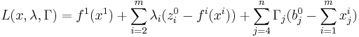
where  and
and  are multipliers.
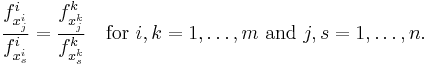
Taking the partial derivative of the Lagrangian with respect to one good, i, and then taking the partial derivative of the Lagrangian with respect to another good, j, gives the following system of equations:
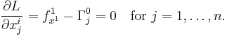
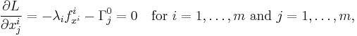
where ƒx is the marginal utility on ƒ' of x (the partial derivative of ƒ with respect to x).
See also
- Admissible decision rule, analog in decision theory
- Bayesian efficiency
- Fundamental theorems of welfare economics
- Constrained Pareto efficiency
- Deadweight loss
- Efficiency (economics)
- Kaldor–Hicks efficiency
- Maximal element, concept in order theory
- Multiobjective optimization
- Nash equilibrium
- Social Choice and Individual Values for the '(weak) Pareto principle'
- Welfare economics
- Game Theory
Notes
- ^ Barr, N. (2004). Economics of the welfare state. New York, Oxford University Press (USA).
- ^ Sen, A. (1993). Markets and freedom: Achievements and limitations of the market mechanism in promoting individual freedoms. Oxford Economic Papers, 45(4), 519–541.
- ^ Ng, 1983.
- ^ Greenwald, Bruce; Stiglitz, Joseph E. (1986). "Externalities in economies with imperfect information and incomplete markets". Quarterly Journal of Economics 101 (2): 229–264. doi:10.2307/1891114. JSTOR 1891114
- ^ Kung, H.T.; Luccio, F.; Preparata, F.P. (1975). "On finding the maxima of a set of vectors.". Journal of the ACM 22 (4): 469–476. doi:10.1145/321906.321910
- ^ Godfrey, Parke; Shipley, Ryan; Gryz, Jarek (2006). "Algorithms and Analyses for Maximal Vector Computation". VLDB Journal 16: 5–28. doi:10.1007/s00778-006-0029-7
References
- Fudenberg, D. and Tirole, J. (1983). Game Theory. MIT Press. Chapter 1, Section 2.4. ISBN 0262061414.
- Ng, Yew-Kwang (1983). Welfare Economics. Macmillan. ISBN 0333971213.
- Osborne, M. J. and Rubenstein, A. (1994). A Course in Game Theory. MIT Press. pp. 7. ISBN 0-262-65040-1.
- Dalimov R.T. Modelling International Economic Integration: an Oscillation Theory Approach. Victoria, Trafford, 2008, 234 pp.
- Dalimov R.T. "The heat equation and the dynamics of labor and capital migration prior and after economic integration. African Journal of Marketing Management, vol. 1 (1), pp. 023–031, April 2009.
- Jovanovich, M. The Economics Of European Integration: Limits And Prospects. Edward Elgar, 2005, 918 p.
- Mathur, Vijay K. "How Well Do We Know Pareto Optimality?" "How Well Do We Know Pareto Optimality?" Journal of Economic Education 22#2 (1991) pp 172–178 online edition